Explore Hillsborough water-quality observations

This tutorial uses the checked Hillsborough EPC water-quality observations layer, a sample view from Hillsborough County monitoring stations rather than region-wide coverage of Tampa Bay. It asks a modest question: how many records contain both reported DO_T and DO_B measurements, and how do those paired values compare? It extends the short paired-reading exploration with an offline source check, a missing-data audit, station and date summaries, and a reproducible ggplot2 chart.

The source is a view of the latest staff-reviewed samples, not a complete monitoring history. The package checks its endpoint and schema; it does not validate laboratory methods or establish measurement units. This is one checked Hillsborough layer, not a survey of all Tampa Bay waters or monitoring programs.

Set up R

Install the package from CRAN and ggplot2 for the optional plotting step. The examples use base R for cleaning and summaries, so ggplot2 is an optional tutorial dependency, not a required package import.

install.packages("tampaBayOpenData")
install.packages("ggplot2")   # if needed for the chart
library(tampaBayOpenData)

The catalog and saved schema chunks below run without a network connection when this article is built. Live chunks are shown but not run during CRAN or website builds. Run those chunks in order in an internet-connected R session to analyze current observations. A source can change or be temporarily unavailable; the retrieval code reports a failure instead of substituting old data.

Find the checked monitoring layer

Search the curated catalog locally. source = "checked" avoids a live portal scan and returns stable package IDs.

library(tampaBayOpenData)

water <- tbod_search_datasets("water quality", source = "checked")
water[, c("id", "title", "publisher", "category", "validation_status")]
#> # A tibble: 1 × 5
#>   id                         title          publisher category validation_status
#>   <chr>                      <chr>          <chr>     <chr>    <chr>            
#> 1 hillsborough-water-quality Hillsborough … Hillsbor… Environ… checked

id <- "hillsborough-water-quality"
info <- tbod_dataset_info(id)
info[c("publisher", "title", "source_url", "verified", "scope_note")]
#> $publisher
#> [1] "Hillsborough County"
#> 
#> $title
#> [1] "Hillsborough EPC water-quality observations"
#> 
#> $source_url
#> [1] "https://hillsborough.maps.arcgis.com/home/item.html?id=04f8f5d7491b4d7aa2aacc6df7ea7f13"
#> 
#> $verified
#> [1] "2026-10-05"
#> 
#> $scope_note
#> [1] "The Environmental Protection Commission's item describes the latest staff-reviewed samples at monitoring stations, not the complete sample history. Methods, units, detection limits, and site coverage require source review."

The verified date marks the catalog’s endpoint check, not a sampling date. The ArcGIS source item is published through Hillsborough County for its Environmental Protection Commission. Read the item’s terms before reusing results; the checked catalog does not identify an unrestricted reuse license for this layer.

Use live discovery to search for other water-related items. A live search depends on portal indexing and does not establish complete regional coverage.

found <- tbod_search_datasets("water quality", source = "live",
                              jurisdiction = "hillsborough", max_items = 10)
found[, c("id", "title", "publisher", "validation_status")]
attr(found, "discovery_complete")

Check fields, locations, dates, and units

The saved layer schema identifies StationNumber and AreaName as location labels, SampleTime as an ArcGIS date field, DO_T and DO_B as numeric fields, and ID as the object ID. Its geometry is a point. These are actual source field names; the saved schema does not provide measurement units or a sampling protocol for the two oxygen fields.

schema <- tbod_schema(id)
needed <- c("ID", "StationNumber", "AreaName", "SampleTime", "DO_T", "DO_B")
stopifnot(all(needed %in% schema$fields$name))
schema$fields[schema$fields$name %in% needed, c("name", "type")]
#> # A tibble: 6 × 2
#>   name          type               
#>   <chr>         <chr>              
#> 1 StationNumber esriFieldTypeString
#> 2 SampleTime    esriFieldTypeDate  
#> 3 AreaName      esriFieldTypeString
#> 4 DO_T          esriFieldTypeDouble
#> 5 DO_B          esriFieldTypeDouble
#> 6 ID            esriFieldTypeOID
schema$geometry_type
#> [1] "esriGeometryPoint"

Inspect the current service metadata before analysis. The package compares it with this bundled baseline again during retrieval and stops on incompatible changes. If source units, depth meanings, or quality-control codes matter to your question, confirm them in the publisher’s current documentation; field names alone are insufficient.

Retrieve and audit current observations

This requests the full current layer with just the fields used here. It checks the retrieval provenance before analysis so a partial result is never treated as a complete view. The request can fail because a service is unavailable, its schema changed, or the operation exceeded its time budget.

current <- tryCatch(
  tbod_dataset_info(id, refresh = TRUE, total_timeout = 90),
  error = function(e) stop("Could not inspect the current EPC layer: ",
                           conditionMessage(e), call. = FALSE)
)
if (!all(needed %in% current$fields$name)) {
  stop("The current EPC layer lacks a field used in this tutorial.",
       call. = FALSE)
}

samples <- tryCatch(
  tbod_get_dataset(id, fields = needed, total_timeout = 240),
  error = function(e) stop("Could not retrieve the complete EPC sample view: ",
                           conditionMessage(e), call. = FALSE)
)
source <- tbod_provenance(samples)
if (!isTRUE(source$complete) ||
    !isTRUE(source$returned_rows == nrow(samples)) ||
    !isTRUE(source$matched_rows == nrow(samples))) {
  stop("EPC retrieval was incomplete; do not interpret these records.",
       call. = FALSE)
}
if (!inherits(samples$SampleTime, c("POSIXct", "Date"))) {
  stop("SampleTime was not returned as a usable date; inspect its time zone metadata.",
       call. = FALSE)
}
source[c("publisher", "source_url", "retrieved_at", "matched_rows",
         "complete", "integrity")]
str(samples[, needed])
head(samples[, needed])

tbod_get_dataset() converts the UTC ArcGIS SampleTime value to an R date-time when the current metadata still declares that time reference. Source column names are preserved. The full retrieval checks object-ID membership, but live attributes can still change during a request.

Clean blank station and area labels, retain only finite numbers for paired measurement calculations, and report exclusions. A missing DO_T or DO_B is not a zero reading.

clean <- data.frame(
  station = trimws(as.character(samples$StationNumber)),
  area = trimws(as.character(samples$AreaName)),
  sample_date = as.Date(samples$SampleTime, tz = "UTC"),
  do_t = as.numeric(samples$DO_T),
  do_b = as.numeric(samples$DO_B)
)
clean$station[is.na(clean$station) | !nzchar(clean$station)] <- NA_character_
clean$area[is.na(clean$area) | !nzchar(clean$area)] <- NA_character_

has_pair <- is.finite(clean$do_t) & is.finite(clean$do_b)
audit <- data.frame(
  check = c("All retrieved records", "Distinct nonblank station IDs",
            "Missing or nonfinite DO_T", "Missing or nonfinite DO_B",
            "Records with both oxygen fields"),
  count = c(nrow(clean), length(unique(stats::na.omit(clean$station))),
            sum(!is.finite(clean$do_t)), sum(!is.finite(clean$do_b)),
            sum(has_pair))
)
print(audit, row.names = FALSE)

paired <- clean[has_pair, , drop = FALSE]
paired$difference <- paired$do_t - paired$do_b

Summarize site coverage and sample dates separately from the oxygen comparison. This is a snapshot of the current view: the month table describes which dates are present, not a trend or a consistent monthly sampling schedule.

station_counts <- sort(table(clean$station, useNA = "no"), decreasing = TRUE)
head(station_counts, 10)

dated <- clean$sample_date[!is.na(clean$sample_date)]
if (length(dated)) {
  range(dated)
  month_counts <- sort(table(format(dated, "%Y-%m")), decreasing = TRUE)
  head(month_counts, 12)
} else {
  message("No sample dates were returned.")
}

areas <- split(paired$difference[!is.na(paired$area)],
               paired$area[!is.na(paired$area)])
if (length(areas)) {
  by_area <- data.frame(
    area = names(areas),
    paired_records = vapply(areas, length, integer(1)),
    median_do_t_minus_do_b = vapply(areas, median, numeric(1))
  )
  by_area <- by_area[order(-by_area$paired_records), , drop = FALSE]
  print(by_area, row.names = FALSE)
} else {
  message("No paired records have a nonblank area label.")
}

The by_area median is a descriptive comparison of the two reported fields, with units unconfirmed. Records may cover stations or dates unevenly; do not rank areas as better or worse water quality from this table.

Plot paired readings

The image below is an archived illustration, generated by the linked exploration from a full layer retrieval on October 6, 2026. It is not a current measurement or the output of this article’s live code. Points on the dashed diagonal have equal reported DO_T and DO_B; points away from it have different values. The original run reported 263 records, of which 161 contained both fields.

Archived October 6, 2026 paired DO_B versus DO_T scatterplot for the Hillsborough EPC station sample view, not region-wide Tampa Bay coverage. A dashed diagonal marks equal reported values.

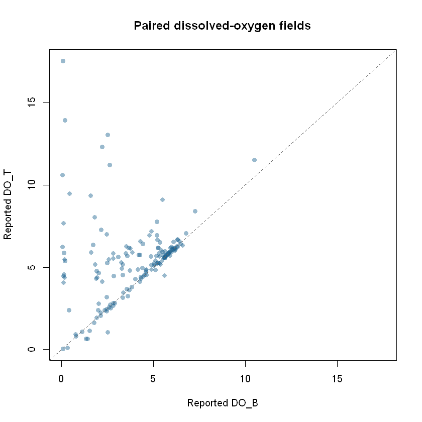
Run this ggplot2 code after the live retrieval to make the same comparison for today’s view. It stops with an informative message if no paired readings are available.

if (!nrow(paired)) {
  stop("No records have both DO_T and DO_B; there is nothing to plot.",
       call. = FALSE)
}
if (!requireNamespace("ggplot2", quietly = TRUE)) {
  stop("Install ggplot2 to draw the oxygen comparison.", call. = FALSE)
}

oxygen_plot <- ggplot2::ggplot(paired, ggplot2::aes(x = do_b, y = do_t)) +
  ggplot2::geom_point(color = "#256789", alpha = 0.55, size = 2) +
  ggplot2::geom_abline(slope = 1, intercept = 0, linetype = "dashed",
                       color = "#555555") +
  ggplot2::coord_equal() +
  ggplot2::labs(
    title = "Paired oxygen fields in the current EPC view",
    subtitle = paste(nrow(paired), "records with both reported values"),
    x = "Reported DO_B (units not confirmed here)",
    y = "Reported DO_T (units not confirmed here)",
    caption = paste("Hillsborough EPC station sample view via tampaBayOpenData;",
                    "not region-wide Bay coverage")
  ) +
  ggplot2::theme_minimal(base_size = 12)
print(oxygen_plot)

Interpret and reproduce the analysis

The chart compares two values within records that report both. Excluded records can differ systematically from included ones. StationNumber and AreaName describe source labels, not independently verified locations; the point layer’s site coverage is not known to be comprehensive. The source view cannot establish historical improvement, regulatory compliance, safety for swimming or drinking, or a cause of any difference. Confirm field units, sampling depths, detection limits, methods, and quality flags with the publisher before making environmental or policy claims.

For a reproducible report, record the output of tbod_provenance(samples), the package version from packageVersion("tampaBayOpenData"), the retrieval time, the fields selected, and the date you consulted the source item. Save the retrieved object and provenance together if you need to revisit a dated analysis. The package does not archive source records.

Continue with housing and development, infrastructure and capital projects, or the Data Coverage dashboard for the checked catalog’s scope and verification status.